Real-time sensor data monitoring is critical for industries ranging from manufacturing to IoT-enabled vehicle sensors for transport. Identifying anomalies, unexpected deviations that could signal equipment failure, environmental hazards, or system inefficiencies, becomes a key challenge when dealing with a stream of sensor readings flowing through a Kafka topic. This blog dives into the process of performing anomaly detection on a set of sensors publishing to a Kafka topic, guiding you through the steps to harness streaming data, apply detection techniques, and ensure timely insights. Whether you’re a data engineer or a curious developer, you’ll discover practical methods to spot the unusual in the constant hum of sensor activity.

Use Case: Missing Data as an Anomaly

For our scenario, we will work with 100 sensors that send a heartbeat every 5 minutes. The sensor is considered down if a heartbeat isn’t detected after 15 minutes. There are two scenarios this leads to: either the sensor is faulty and is sending heartbeats after the window, or it stops sending a heartbeat entirely. To simulate this data, I wrote a Python program with the following parameters:

  • 100 sensors comprised of:
    • UUID as a sensor ID
    • Unix epoch timestamp
    • Generate sensor records for 100 days starting from November 1, 2024
  • Each sensor will start at random times over 48 hours from the start date
  • 10% of the sensors will fail to generate a timestamp for a random amount of time between 15 and 120 minutes on a random number of days
  • 2% of the sensors will stop sending a timestamp between 15 and 60 days from the first timestamp.

Here is the Python code if you want to play with it yourself in a free DeltaStream trial; you just need a Kafka cluster of your own available:

  1. import json
  2. import time
  3. import random
  4. import uuid
  5. import datetime
  6. from kafka import KafkaProducer
  7.  
  8. # Kafka Configuration
  9. KAFKA_BROKER = "your bootstrap server"
  10. TOPIC = "sensor_data"
  11.  
  12. # Kafka Producer Setup
  13. producer = KafkaProducer(
  14. bootstrap_servers=KAFKA_BROKER,
  15. security_protocol='SASL_SSL',
  16. sasl_mechanism='SCRAM-SHA-512',
  17. sasl_plain_username='your username',
  18. sasl_plain_password='your password',
  19. value_serializer=lambda v: json.dumps(v).encode("utf-8"),
  20. key_serializer=lambda k: k.encode("utf-8") if k is not None else None,
  21. )
  22.  
  23. # Simulation Constants
  24. SENSOR_COUNT = 100
  25. TEMP_FAILURE_PERCENTAGE = 0.10 # 10% of sensors fail randomly
  26. PERM_FAILURE_PERCENTAGE = 0.02 # 2% of sensors fail permanently
  27. INTERVAL_SECONDS = 5 * 60 # 5 minutes
  28. TEMP_FAILURE_MIN = 15 * 60 # 15 minutes
  29. TEMP_FAILURE_MAX = 120 * 60 # 120 minutes
  30. PERM_FAILURE_MIN_DAYS = 15 # 15 days
  31. PERM_FAILURE_MAX_DAYS = 60 # 60 days
  32. START_DATE = datetime.datetime(2024, 11, 1, 0, 0, 0)
  33. SIMULATION_DAYS = 100
  34. SIMULATION_DURATION = SIMULATION_DAYS * 24 * 60 * 60 # 100 days in seconds
  35. RANDOM_START_WINDOW = 48 * 60 * 60 # 48 hours in seconds
  36.  
  37. # Generate 100 Unique Sensor IDs
  38. sensors = [str(uuid.uuid4()) for _ in range(SENSOR_COUNT)]
  39.  
  40. # Select 10% of sensors for temporary failures
  41. temp_fail_sensors = set(random.sample(sensors, int(SENSOR_COUNT * TEMP_FAILURE_PERCENTAGE)))
  42.  
  43. # Select 2% of sensors for permanent failures
  44. perm_fail_sensors = set(random.sample(sensors, int(SENSOR_COUNT * PERM_FAILURE_PERCENTAGE)))
  45.  
  46. # Assign each sensor a random start time within the first 48 hours
  47. sensor_start_times = {
  48. sensor: START_DATE.timestamp() + random.randint(0, RANDOM_START_WINDOW)
  49. for sensor in sensors
  50. }
  51.  
  52. # Generate failure windows (15-120 min) for temporary failures
  53. temp_fail_windows = {}
  54. for sensor in temp_fail_sensors:
  55. num_failures = random.randint(3, 10) # Number of random failure periods
  56. failure_days = random.sample(range(1, SIMULATION_DAYS + 1), num_failures)
  57.  
  58. temp_fail_windows[sensor] = [
  59. (
  60. START_DATE.timestamp() + (day * 24 * 60 * 60) + random.randint(0, 24 * 60 * 60),
  61. START_DATE.timestamp() + (day * 24 * 60 * 60) + random.randint(0, 24 * 60 * 60) + random.randint(TEMP_FAILURE_MIN, TEMP_FAILURE_MAX)
  62. )
  63. for day in failure_days
  64. ]
  65.  
  66. # Assign permanent failure times (between 15 and 60 days from start)
  67. perm_fail_times = {
  68. sensor: sensor_start_times[sensor] + random.randint(PERM_FAILURE_MIN_DAYS * 24 * 60 * 60, PERM_FAILURE_MAX_DAYS * 24 * 60 * 60)
  69. for sensor in perm_fail_sensors
  70. }
  71.  
  72. # Track permanently failed sensors
  73. perm_failed_sensors = set()
  74.  
  75. # Track last failure timestamp for each sensor (prevents duplicate logs)
  76. last_fail_timestamp = {sensor: None for sensor in temp_fail_sensors}
  77.  
  78. # Start simulation at the given start date
  79. current_time = START_DATE.timestamp()
  80.  
  81. while current_time <= START_DATE.timestamp() + SIMULATION_DURATION:
  82. for sensor in sensors:
  83. start_time = sensor_start_times[sensor]
  84.  
  85. if current_time >= start_time:
  86. # Check if the sensor has permanently failed
  87. if sensor in perm_fail_sensors and current_time >= perm_fail_times[sensor]:
  88. if sensor not in perm_failed_sensors:
  89. print(f"❌ Sensor {sensor} permanently stopped at {datetime.datetime.utcfromtimestamp(perm_fail_times[sensor])}")
  90. perm_failed_sensors.add(sensor)
  91. continue # Sensor is permanently down
  92.  
  93. # Check if the sensor is temporarily failing
  94. if sensor in temp_fail_sensors:
  95. for fail_start, fail_end in temp_fail_windows[sensor]:
  96. if fail_start <= current_time <= fail_end:
  97. if last_fail_timestamp[sensor] != fail_start:
  98. print(f"⚠️ Sensor {sensor} temporarily down from {datetime.datetime.utcfromtimestamp(fail_start)} to {datetime.datetime.utcfromtimestamp(fail_end)}")
  99. last_fail_timestamp[sensor] = fail_start # Prevent duplicate logs
  100. continue # Skip sending data
  101.  
  102. # Normal sensor data (only sensor_id and timestamp)
  103. data = {
  104. "sensor_id": sensor,
  105. "time_stamp": int(current_time) # Use integer UNIX timestamp for clarity
  106. }
  107.  
  108. # Send data to Kafka
  109. producer.send(TOPIC, value=data, key=sensor)
  110.  
  111. # Move simulation time forward by 5 minutes
  112. current_time += INTERVAL_SECONDS
  113.  
  114. # Close producer after all data is sent
  115. producer.close()

Our resulting JSON file looks like this:

  1. {
  2. "key": {
  3. "key": "268aded0-0cd4-49ce-ab49-cfc123fdabf9"
  4. },
  5. "value": {
  6. "sensor_id": "268aded0-0cd4-49ce-ab49-cfc123fdabf9",
  7. "time_stamp": 1730447400
  8. }
  9. }

Solution: Detecting failed Sensors

All of the SELECT statements are displayed in the following screenshot, as well as some of the results of glitching sensors and the number of minutes they failed to send their heartbeat. 

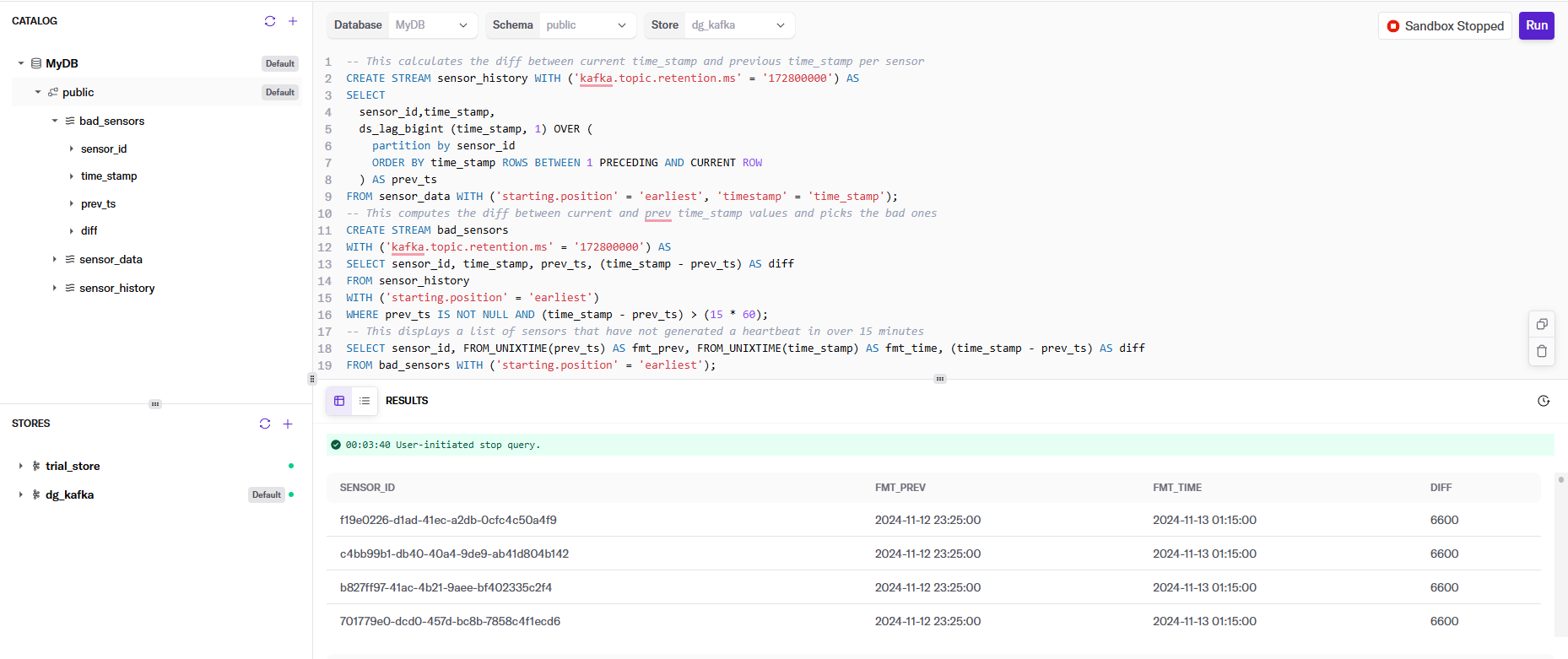
Let’s break down each of the statements and explain what we’re doing:
This first statement creates a DeltaStream Object of type STREAM that defines the layout of the sensor_data topic in our Kafka cluster. This gives us an entity that we can perform actions on against the topic.

  1. CREATE STREAM sensor_data (
  2. sensor_id VARCHAR, time_stamp BIGINT )
  3. WITH ('topic' = 'sensor_data', 'value.format' = 'json');

This part has the secret sauce to making this work: the ds_lag_bigint function. It is a built-in function to access the value of a column from a previous row within the same relation. This is particularly useful for scenarios where you need to compare or compute differences between rows. In our case, we use it to determine the time interval between consecutive sensor events. The function requires specifying the column from which to retrieve values and the number of rows from which to look back. For example, ds_lag_bigint(time_stamp, 1) returns the time_stamp from the previous row, allowing us to calculate the time difference between consecutive sensor readings and thus determine if the difference is outside our acceptable bound of 15 minutes.
Other than that, we’re creating the stream topic with a retention of 72 hours (in milliseconds) to ensure the data lasts long enough to run my tests. Finally, the FROM clause forces the SELECT to read from the beginning of the topic, and what field is the timestamp.

  1. -- This calculates the diff between current time_stamp and previous time_stamp per sensor
  2. CREATE STREAM sensor_history WITH ('kafka.topic.retention.ms' = '172800000') AS
  3. SELECT
  4. sensor_id,
  5. time_stamp,
  6. ds_lag_bigint (time_stamp, 1) OVER (
  7. partition by sensor_id
  8. ORDER BY time_stamp ROWS BETWEEN 1 PRECEDING AND CURRENT ROW
  9. ) AS prev_ts
  10. FROM
  11. sensor_data WITH ('starting.position' = 'earliest', 'timestamp' = 'time_stamp');

Next, we create a new Kafka Topic, bad_sensors, for any record in sensor_history with two timestamps greater than 15 minutes. This will be our list of sensors with anomalies that need to be researched. If they go online and offline outside of our acceptable range, they are likely failing, or something else needs to be investigated.

  1. -- This computes the diff between current and prev time_stamp values and picks the bad ones
  2. CREATE STREAM bad_sensors
  3. WITH
  4. ('kafka.topic.retention.ms' = '172800000') AS
  5. SELECT
  6. sensor_id,
  7. time_stamp,
  8. prev_ts,
  9. (time_stamp - prev_ts) AS diff
  10. FROM
  11. sensor_history
  12. WITH
  13. ('starting.position' = 'earliest')
  14. WHERE
  15. prev_ts IS NOT NULL
  16. AND (time_stamp - prev_ts) > (15 * 60);

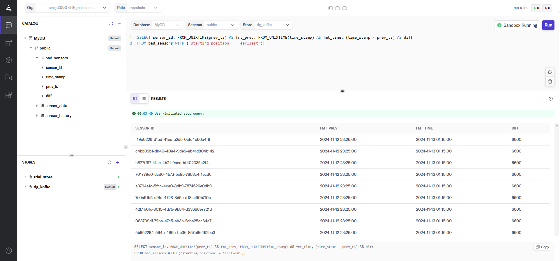
Finally, let’s take a look at the data in bad_sensors. This formats out the current and previous heartbeat timestamps and the difference between them in minutes.

  1. SELECT
  2. sensor_id,
  3. FROM_UNIXTIME(prev_ts) AS fmt_prev,
  4. FROM_UNIXTIME(time_stamp) AS fmt_time,
  5. (time_stamp - prev_ts) AS diff
  6. FROM
  7. bad_sensors
  8. WITH
  9. ('starting.position' = 'earliest');

In a production environment, it would make sense for the bad_sensors data to be fed into a location that populates a dashboard where decisions can be made in near real-time. This could be something like Iceberg, Clickhouse, Databricks, Snowflake, or whatever you use.

Summary

This blog explores anomaly detection for real-time sensor data on a Kafka topic, using a 100-sensor setup with heartbeats every 5 minutes. We define anomalies as misses exceeding 15 minutes, simulate 100 days of data with Python, and apply DeltaStream to process it, racking history, calculating gaps with ds_lag_bigint, and pinpointing failures via SQL. This approach is streamlined for engineers and easily adaptable to production dashboards.