22 Apr 2025
Min Read
Enable “Shift-Left” with Apache Kafka and Iceberg
In the past few years, the Apache Iceberg table format has become the 800-pound gorilla in the data space. DeltaStream supports reading and writing Iceberg using either the AWS Glue catalog or the Apache Polaris (incubating) catalog. This blog walks you through a data scenario in which data in Apache Kafka topics are read, filtered, and enriched with data from another Kafka topic, then written to Iceberg and queried from DeltaStream.
Writing Data Tables to Iceberg
When you sign up for a DeltaStream demo, you’re provided with a demo Kafka cluster called trial_store. If you are unfamiliar with DeltaStream, this short interactive demo walks you through it. For the Iceberg catalog implementation, we’ll be using REST and the Snowflake Polaris implementation, the docs for which can be found here. AWS Glue is also supported, as is any other REST implementation.
For this example, we’ll use two of the topics in that cluster and follow the first part of the Quick Start guide, but we’ll enhance it to write two new tables of processed data to Iceberg.
Our demo includes the following:
- Users Kafka topic
- Pageviews Kafka topic
- Enrich the pageviews with user information
- Write to two tables in Iceberg, comprised of:
- Pageviews per city per minute
- Pageviews per user per hour
Our queries do the following:
- Top 3 cities with highest pageviews per hour
- Top 5 users with the highest pageviews per hour
Streaming Lakehouse with DeltaStream Fusion
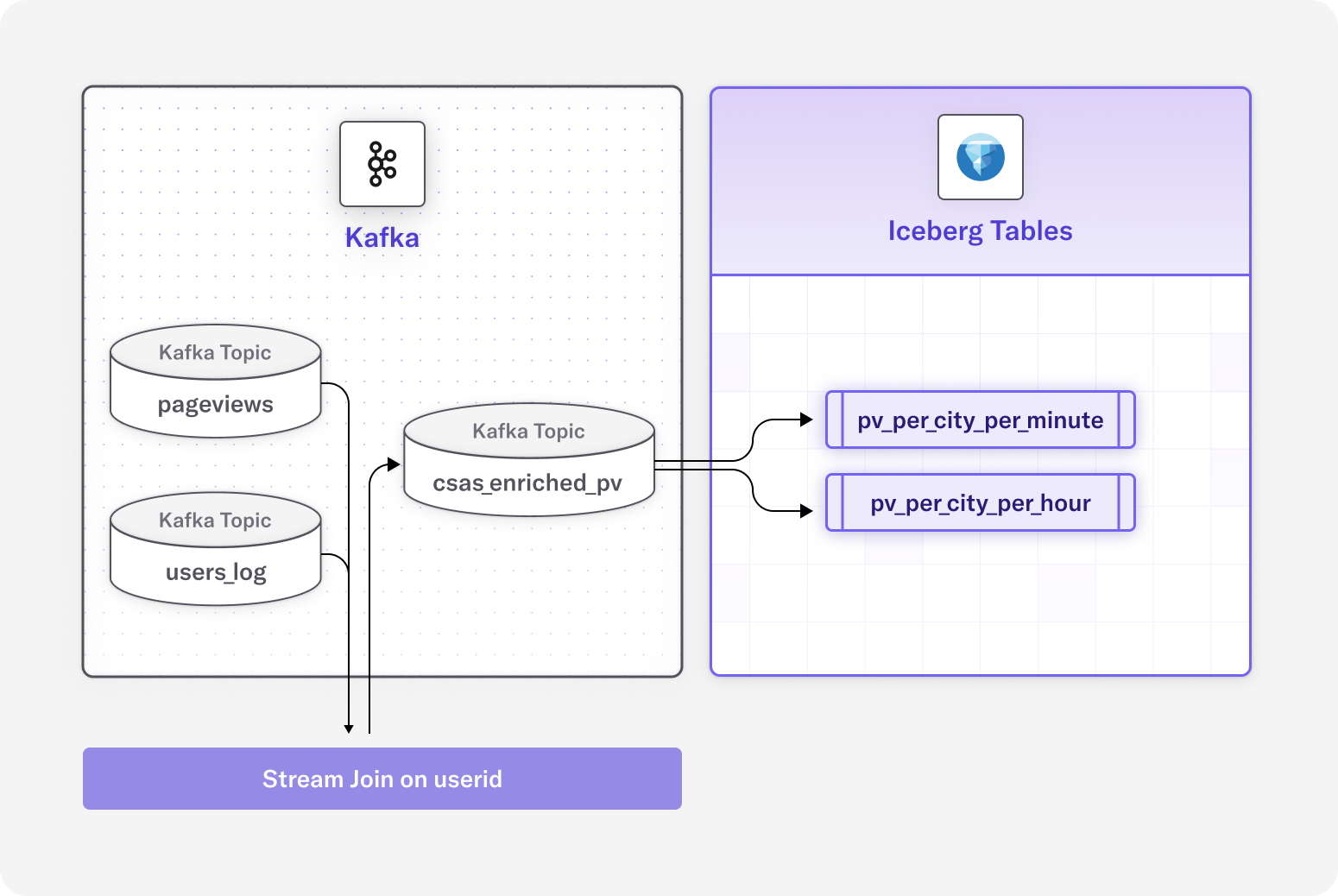
First, let’s define the data we are working with. Our Kafka topic pageviews looks like this:
That means we need to create a DeltaStream, Stream-type Object. We do this with a CSAS statement:
That now sets up our pageviews topic so you can access it via SQL. Let’s look at the data structure in our users topic. Note that a userid field will tie the two streams together.
Next, we define a DeltaStream Changelog object for our users topic named users_log. Note that we’ve created an array from interests and a struct from the contactinfo. Also note that state is a reserved word in DeltaStream, so it is enclosed in quotes. Our command looks like this:
Next, we join our STREAM and CHANGELOG into a new enriched Kafka topic defined as a DeltaStream STREAM object named csas_enriched_pv. This combines user data with the pageviews information that is written to our Iceberg table.
Here is what that data looks like for reference:
Now that the Kafka topic csas_enriched_pv is available, the fun part begins. This creates an Iceberg table with our “Pageviews per state per minute” scenario. If you are unfamiliar with configuring Iceberg in DeltaStream, this short interactive demo can walk you through it.
Let’s break down what is happening here for those unfamiliar:
- CREATE TABLE pv_per_city_per_minute: Creates a new table named "pv_per_city_per_minute"
- WITH(...): Contains table properties or configurations. Further explanation is below.
- SELECT user_city, count(pageid) AS viewcount, window_start, window_end:
- Selects the user's city
- Counts the number of page IDs and names this count "viewcount"
- Includes the start and end times of each window interval
- TUMBLE(csas_enriched_pv, size 1 minutes): Applies a tumbling window function to the "csas_enriched_pv" table with a window size of 1 minute. A tumbling window divides data into non-overlapping, fixed-size time intervals.
- GROUP BY user_city, window_start, window_end: Groups the results by state and time window, so the count is calculated separately for each state within each one-minute interval
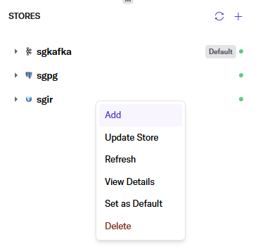
One possible initial confusion is where that ‘iceberg.rest.catalog.namespace.name’ value comes from. Iceberg supports an arbitrary number of namespaces to organize tables in a catalog. Our data store that maps to the Iceberg catalog is named sgir; by right-clicking on it we get a dialog that includes add, which prompts for a name. This becomes your new namespace; in our case, it is sgns.
To further explain the WITH parameters, the ‘iceberg.rest.catalog.table.name’ specifies the same value as the CREATE TABLE. It can be a different value to alias the table name you’ll be using in your queries to the table in Iceberg – for example, if you want to shorten the name or organize your query in a particular fashion. In our case, though, we’re keeping the values the same.
With that query running, let’s launch our second query to generate our table for “Pageviews per user per hour.” What we’re doing here is very similar, but we’ve changed our TUMBLE window to 1 hour and are using userid instead of user_city.
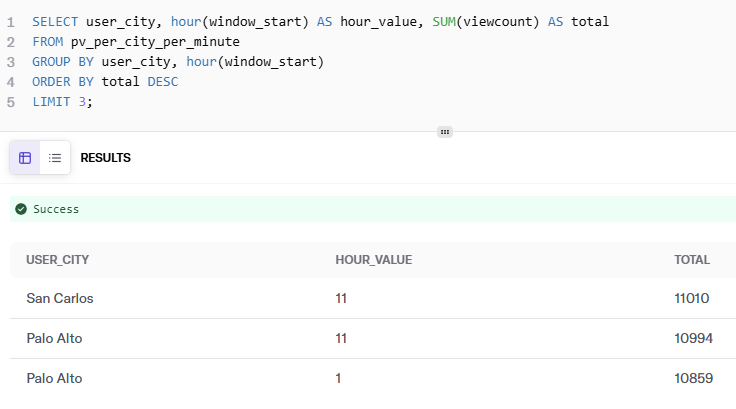
Without leaving DeltaStream, we can query the Iceberg table for our “Pageviews per city per minute” scenario directly in the same workspace and get results without moving to another tool.
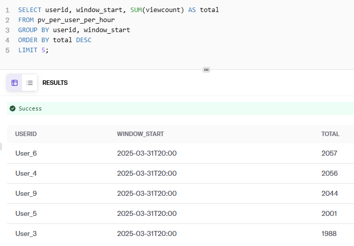
Next, we perform our second query to get the results from our Iceberg table for our top 5 users per hour.
Like our first scenario, our second scenario, “Pageviews per user per hour, " is all within DeltaStream. Since this data is now in Iceberg, you can also use any other compatible compute engine or BI tool without any lock-in.
Shift-left and So Much More
We’ve just walked through a classic “shift-left” scenario where we have moved enrichment and filtering to the streaming architecture and the popular Iceberg table format on AWS, making it available to query from any compatible compute engine. We’ve reduced latency by not waiting for a batch process to move the data through a medallion architecture, and we’ve reduced costs by eliminating that transformation compute cost and additional storage. We can even query those Iceberg tables from DeltaStream to do additional joins and enhancements and write them back out to Iceberg if we want. This is just the tip of the, um, Iceberg when it comes to what is possible with DeltaStream.